
 |
| You may not know it, but today is epic. It is the last day for John Stockwell who is retiring out of the Colorado School of Mines after 42 years. John is an amazing guy that I have been lucky enough to call a friend since 1986. Mathematician, programmer, geophysicist, keeper of SeismicUnix; a multifaceted man who can just as easily discuss Pythagoras or python programming, always delivered with a zesty sense of humor. The photo is from the editors dinner at the 2015 SEG annual meeting in New Orleans where a very pleasant Presidential duty for me was to give the SEG wiki Champion award to John. Good luck after CSM John! |
Thursday, December 21, 2017
Stockwell Retires
Saturday, December 9, 2017
Disc 22 Buenos Aires (10 August)
Encore repost from THURSDAY, AUGUST 16, 2012
———-
Buenos Aires is a wonderful place and the people are friendly beyond measure. Special thanks need to go out to Gutavo Carstens who picked me up at the airport and coordinated a watch party for the Olympic basketball game between USA and Argentina. Another big shout-out to the very kind Patricio (Patrick) Marshall who introduced me to the city, marked many interesting things on a city map, and urged me to go to the street market held each Sunday near San Telmo.
The DISC was well-attenend and held in the stunning YPF office tower overlooking the city. Thanks to all!

The Buenos Aires DISC 2012 class. Bearded guys in the back: Gustavo (center) and Patrick (right)
If you come to Buenos Aires, and I hope you will, there is much to see and do. But I want to tell you about just one. It is a plea, a screaming rant of recommendation. It is the best meal I have ever had, and that is saying something. My wife makes meals 4 times a week that are better than anything most men ever taste. I've dined all over Spain, in Italy, France, and dozens of other countries. In short, I have had a lot of great meals. But the Buenos Aires restaurant Dora stands alone.
I'm not a food critic, but I know what one should say about Dora. Not all of Buenos Aires is nice, not all of it safe. But step into Dora and feel a waft of the old times, where waiters watch patrons closely (but not obsessively) to anticipate what is needed next; real waiters who do it for a living and have for generations. No pretension, no haughty indifference, no demeaning glances. A pride in trade and work that the modern world has long forgotten. If this were all, there would be other contenders. But then comes the food. For starters I had grilled langostinos (thin rock lobsters) halved in a beautiful sauce. Then came the Cazuela Dora, a house special seafood stew with saffron rice on the side. It was a symphony, not the drippy rehash kind of symphony nodding to the real thing, or a quirky modern symphony that is little more than a jumble of noise aimed at glorifying the sad creatures who write and direct it. No this was an old school, honest symphony of taste. A fragment, a remnant of the guilded age when a symphony was a symphony and if you wrote one you had damn well better get it right or be out of a job. The food spilled over an ample plate, the wine, of course, was malbec, rich and full-bodied and lots of it. I ate until I could eat no more, then ate more. The waiter tried to clear the table a couple of times, but I would have nothing to do with it. I did not want the meal to end. Finally, reluctantly, regretfully, with remorse I let it go.
I know what the food critic should say about Dora, but this is a tainted age of tiny multicolor pyramids parading as food on vast plates with artistic drizzles of sauce, a time when the chef is a reality TV star and a lacky runs the kitchen. Yep, I know what the critic should say, but have no faith it will ever be said. Go to Buenos Aires, go to Dora, eat, live.
Monday, December 4, 2017
Basecamp
Like many academics, I have many things going on and it is easy to get them mixed up or have something important get dropped. I keep a todo list on paper and one on the board in my office, that helps with the daily buzz of Department Chair duties. But the main bottleneck is students that I advise, a group consisting of 1 undergraduate honors, 8 masters and 1 PhD candidate. Each has a committee, sometimes more than one. Our PhD students, for example, have a candidacy exam committee and a thesis committee which may, or may not, consist of the same individuals. Easy to miss something in that quagmire.
But then I heard about Basecamp_3, or just basecamp, from email traffic on the SEG Research Committee. For several years there have been efforts to establish a networking environment using SEG internal IT resources. But it is a big job and a moving target with several commercial or free alternatives. The research committee is experimenting with basecamp and so am I. My first impression is very positive.
For academic users, basecamp is free after you jump through a few hoops to prove you are academic. Not a big deal, but it is there. Basecamp was developed for business use to give "a 10,000 ft view of everything that's happening across your whole business." Imagine a not-so-small company with teams and projects shown organized into a snazzy web layout and you have a first understanding of basecamp. The elements of each project are customizable, but usually contain a message board, schedule, todo list and documents area. Unlike group emails, the messages and responses are permanently archived in an easily accessible form with full history. The todo items point at one or many individuals, but everyone in the project sees the todo items for everyone.
 On 21 September of 2017 I jumped in to basecamp with the goal of organizing the students I advisees, their committees, deadlines, documents and todo lists. To the left is a screenshot of my basecamp as it appears today. At the top is my headquarters (Prof. Liner HQ) where announcements can be made that everyone in the tree will get. Very dangerous power, use it sparingly. The only team I maintain are my advisees so that I can communicate common information to all of them at once. In the projects area, each student is a project, either honors (HON), masters (MS) or doctorate (PhD). The small dots with initials are people associated with a project; the student, the advisor (me) and the committee. One MS student has two ex-officio members from Houston who are also able to keep with with progress via basecamp.
One project is experimental: we are using it to organize the departmental geology curriculum committee that is looking at an overhaul of undergraduate and MS requirements. Early indications are also good for this use.
Inside a particular student project are the elements shown in the figure below. A nice feature of basecamp is insulation of each project from all the others. Project chatter is confined to the members of that project and is well organized. Notice the schedule items show up in the project view; no more drilling down into calendars with items for all students to find out what is coming up for a particular student.
We have developed a method for thesis revisions that works beautifully within basecamp. At the early stages, the student composes a complete chapter and posts it to basecamp for advisor review. This is an MS Word document that is edited with track changes on. Figure call-outs are in the text, but the actual figures do not reside in the word file. Figures are in an MS Powerpoint file with one slide for each figure and caption in the notes area of that slide. Let's say the files are SmithMSChap1_R1.docx (text) and SmithMSChap1_R1.pptx (figures). When the advisor has edited both, they are reposted to basecamp using the nifty feature that a file can be replaced with an updated version by anyone on the project member list and all the previous comments remain in place as a history file. In this case, I would replace SmithMSChap1_R1.docx with SmithMSChap1_R2.docx and use the same convention for the figures file. After each committee member has reviewed R2 (and possibly uploaded R3), then we move on to the next chapter. After this process, all the chapters are pulled together into SmithMSThesis_R1.docx and the review process iterates to conclusion.
 The documents area allows creation of folders to hold related material, so you can have folders such as Proposal, Thesis, Defense, etc. It is hard to see how I kept it all straight before basecamp, but I do not want to go back to that time of chaos and confusion.
 Wednesday, November 15, 2017
Chair Top 10 List
I have been Chair of the Department of Geosciences at the University of Arkansas for about a year-and-a-half now. For what it is worth, here is my top 10 list of advice for new Chairs:
Make a list of deadlines, mine has about 150 items
Support, expand and involve your external advisory board - they can move the world
Every time you complete a complicated task, write a note titled "for next time" about how you could do it better
Start a blog to capture all the stuff you need to share,here is mine
Choose committee members carefully, dysfunctional committees are bad news
Make a 4-year teaching plan for the department, here is mine
Put together an advisory group of senior faculty
Mainly watch and learn for a year, then initiate change where needed
Clarify, streamline and simplify processes
Communicate and delegate
Wednesday, November 8, 2017
Simon Klemperer
Dear Prof. Liner:
I just wanted to take a break from updating my lectures on migration to say how much I am enjoying “Elements” to teach my Reflection Seismology class. Beautifully clear, with an original take on numerous concepts and very different in philosophical approach from a more “conventional” text like Sheriff & Geldart.

But I had to go online to find your contact info, and because I have a butterfly mind I also now have a .pdf of Greek Seismology and encourage you, should there be a v. 2.1, to correct the typo on page 6: “There was also earlier experimental work by Hook, Galileo and others” to give Hooke his due terminal e (he does indeed feature in my lectures for “ut tensio, sic vis”)
And finally, I am intrigued by Spice: is it available for academics to play with? One of my students is making seismic-stratigraphic interpretations, and I would be fascinated to see whether anything new came out of the data.
Regards,
Simon Klemperer
~~~~~~~~~~~~~~~~~~~~~~~~~~~~~~
Simon Klemperer
Professor of Geophysics, and of Geological Sciences
Department of Geophysics, Stanford University,
Mitchell Building 353, 397 Panama Mall, Stanford CA 94305-2215
telephone: (650) 723 8214 (department manager: 498-6877) fax : (650) 725 7344
sklemp@stanford.edu https://pangea.stanford.edu/
http://scholar.google.co.uk/
~~~~~~~~~~~~~~~~~~~~~~~~~~~~~~
==================
Dear Simon,
Thank you for the very kind note. It is not often that one gets such a complimentary email. So glad you are enjoying the Elements book, I assume you are reading the 3rd edition. It is much improved from the 2nd edition.
I would love to make the correction you mention to the Earthquake book. But, alas, the source file is in word 6 or word 95 (which may be the same thing), and current Word versions will not open it. So we are stuck with the PDF only.
Yes, spice will be available in the next release of seismic unix. The source file is attached. If you are familiar with SU, adding this to your install should not be too much trouble. A typical processing flow would go like this:
succwt < in_su_data fmax=100 noct=5 nv=10 \
| suspice seth=1 amax=35 amin=1,5,10 ta=0,2,4 > out_spice_data
Hope you find spice useful. I have found it takes very good quality data before spice works well. But when it works, it is remarkable.
Best regards,
Chris
ps. If you don't mind, I'll post your letter and my response to my seismos blog.
Thursday, October 26, 2017
A nice note
Got this note today from a recent graduate of the U Arkansas Geosciences Department:
Hello Dr Liner,
I hope this email finds you well. I was hired and currently working for an environmental consulting company ECS Mid-Atlantic as an environmental technician. The recommendation you provided on my application went a long way in helping me secure this position.
The project I am currently assigned to is focused on environmental remediation of a coal ash pond from Dominion Power Company. In my role as a technician, I run lab tests checking the quality of the water being treated and report to the site supervisor when the water quality drops.
I plan on being in this position for a while and hopefully continuing to graduate school with this experience.
Thank you all your help and have a great day.
Yours Sincerely,
Asher S.
----------- my reply ----------------------
Hi Asher,
What a wonderful note! Thank you for letting me know about your new career. I will share this with the new Careers class I am teaching that meets tonight. Several of the students know you.
Continued good luck and best regards,
Prof. Christopher L. Liner
Department of Geosciences Chairman
Storm Endowed Chair of Petroleum Geology
University of Arkansas
Thursday, October 12, 2017
Python easy earth globe
You can make a stunning earth globe, including topography and bathymetry, with just a few lines of python. Just now, I am interested in New Zealand, so we can put it in the middle. Here is the code:
from mpl_toolkits.basemap import Basemap
import matplotlib.pyplot as plt
import numpy as np
map = Basemap(projection='ortho', lat_0=-30, lon_0=170, resolution='l')
map.etopo()
map.drawcountries()
map.drawmeridians(np.arange(0,360,30))
map.drawparallels(np.arange(-90,90,30))
plt.show()

from mpl_toolkits.basemap import Basemap
import matplotlib.pyplot as plt
import numpy as np
map = Basemap(projection='ortho', lat_0=-30, lon_0=170, resolution='l')
map.etopo()
map.drawcountries()
map.drawmeridians(np.arange(0,360,30))
map.drawparallels(np.arange(-90,90,30))
plt.show()
Below is the result, not bad for 9 lines of code!

Thursday, April 27, 2017
Python, wells, LAS and info
Those of you who deal with wireline well log data know that the standard format is call LAS. A nice site from the Canadian Well Logging Society that explains the format can be found here. In the old days, a well would be logged for gamma ray, density and maybe a couple of electric logs. In today's world, a full logging assault can yield a vast collection of data types (called curves). Not only that, but these might be split across many LAS files. One well in our data base has 17 LAS files! Each individual curve has a short abbreviation (a mnemonic) such as GR (gamma ray), RHOB (bulk density) and DT (compressional sonic). The mnemonics are somewhat standardized, but in fact there is broad variability between logging companies. Each curve also has units and a description field in the LAS file.
How do you figure out what curves are contained in such a collection of LAS files? Well, one approach is to convert each LAS to an excel file, but that gets messy and brings in the data as well as the curve information. The Agile Geoscience folks have discussed this topic and python in detail; here we have a less ambitious goal that allows a simple solution.
To deal with this problem, I wrote a code in python that I call info.py - here it is
This little code is magic, mainly because it draws on lasio, a library for reading and writing LAS files. Stepping through the code line-by-line goes like this
I work on a mac which has a command line terminal and python build in. Python has lots of default libraries, but others are always needed. I install them with pip, but first you must install pip itself
sudo easy_install pip
Then this command line installs lasio
sudo pip install lasio
How do you figure out what curves are contained in such a collection of LAS files? Well, one approach is to convert each LAS to an excel file, but that gets messy and brings in the data as well as the curve information. The Agile Geoscience folks have discussed this topic and python in detail; here we have a less ambitious goal that allows a simple solution.
To deal with this problem, I wrote a code in python that I call info.py - here it is
import lasio
import os
n = 1
for file in os.listdir("."):
if file.endswith(".las") or file.endswith(".LAS"):
var = lasio.read(file)
print "\n las"+str(n), file
print var.well
print var.other
for curve in var.curves:
print("%s\t[%s]\t%s\t%s" % (curve.mnemonic, curve.unit, curve.value, curve.descr))
n += 1
- import the lasio library
- import the operating system library
- set counter n to 1
- for each file in the current directory...
- if the file name ends in las or LAS...
- read the file
- print 'las' with n appended, then the file name
- print the 'well' data section of the file
- print the 'other' data section of the file
- for each curve in the file print mnemonic, units, value and description
- increase n by 1 and continue till all files are read
I work on a mac which has a command line terminal and python build in. Python has lots of default libraries, but others are always needed. I install them with pip, but first you must install pip itself
sudo easy_install pip
Then this command line installs lasio
sudo pip install lasio
Now you are ready to go. The code above can be copied into a text editor and saved as info.py (or another name you like better). Now go to a directory full of LAS files from a well and copy info.py into that folder. On the mac, open a terminal window and cd to the LAS directory, then type
python info.py
or, if you want to capture the output into a file
python info.py > info_jones1a.txt
The result will look something like the listing at the end of this post. The beauty of this little code fragment is the amount of information it makes readily available in complex well situations with many, or redundant, or overlapping LAS files.
Hope you enjoy the code and it helps you organize a few tough LAS situations.
las1 Jones_1A_run1.las
Mnemonic Unit Value Description
-------- ---- ----- -----------
STRT F 437.0 START DEPTH
STOP F 4000.5 STOP DEPTH
STEP F 0.5 STEP
NULL -999.25 NULL VALUE
COMP Jones COMPANY
WELL 1A WELL
FLD WILDCAT FIELD
LOC SHL: 1320' FNL & 2210' FWL LOCATION
CNTY COUNTY
STAT STATE
CTRY COUNTRY
SRVC SERVICE COMPANY
API API NUMBER
DATE 8-Jun-2012 LOG DATE
UWI UNIQUE WELL ID
DEPT [F] DEPTH (BOREHOLE) {F12.4}
C1 [IN] Caliper 1 {F11.4}
C2 [IN] Caliper 2 {F11.4}
CDF [LBF] Calibrated Downhole Force {F11.4}
CTEM [DEGF] Cartridge Temperature {F11.4}
DCAL [IN] Differential Caliper {F11.4}
DEVI [DEG] Hole Deviation {F11.4}
GR_EDTC [GAPI] EDTC Gamma Ray {F11.4}
GTEM [DEGF] Generalized Borehole Temperature {F11.4}
HAZI [DEG] Hole Azimuth {F11.4}
HAZIM [DEG] Hole Azimuth {F11.4}
P1AZ [DEG] Pad 1 Azimuth {F11.4}
RB [DEG] Relative Bearing {F11.4}
SDEV [DEG] Sonde Deviation {F11.4}
SDEVM [DEG] Sonde Deviation {F11.4}
STIT [F] Stuck Tool Indicator, Total {F11.4}
TENS [LBF] Cable Tension {F11.4}
las2 Jones_1A_run2.las
Mnemonic Unit Value Description
-------- ---- ----- -----------
STRT F 437.0 START DEPTH
STOP F 4000.5 STOP DEPTH
STEP F 0.5 STEP
NULL -999.25 NULL VALUE
COMP Jones COMPANY
WELL 1A WELL
FLD WILDCAT FIELD
LOC SHL: 1320' FNL & 2210' FWL LOCATION
CNTY COUNTY
STAT STATE
CTRY COUNTRY
SRVC SERVICE COMPANY
API API NUMBER
DATE 8-Jun-2012 LOG DATE
UWI UNIQUE WELL ID
DEPT [F] DEPTH (BOREHOLE) {F12.4}
AF10 [OHMM] Array Induction Four Foot Resistivity A10 {F11.4}
AF20 [OHMM] Array Induction Four Foot Resistivity A20 {F11.4}
AF30 [OHMM] Array Induction Four Foot Resistivity A30 {F11.4}
AF60 [OHMM] Array Induction Four Foot Resistivity A60 {F11.4}
AF90 [OHMM] Array Induction Four Foot Resistivity A90 {F11.4}
AO10 [OHMM] Array Induction One Foot Resistivity A10 {F11.4}
AO20 [OHMM] Array Induction One Foot Resistivity A20 {F11.4}
AO30 [OHMM] Array Induction One Foot Resistivity A30 {F11.4}
AO60 [OHMM] Array Induction One Foot Resistivity A60 {F11.4}
AO90 [OHMM] Array Induction One Foot Resistivity A90 {F11.4}
AT10 [OHMM] Array Induction Two Foot Resistivity A10 {F11.4}
AT20 [OHMM] Array Induction Two Foot Resistivity A20 {F11.4}
AT30 [OHMM] Array Induction Two Foot Resistivity A30 {F11.4}
AT60 [OHMM] Array Induction Two Foot Resistivity A60 {F11.4}
AT90 [OHMM] Array Induction Two Foot Resistivity A90 {F11.4}
AHFCO60 [MM/M] Array Induction Four Foot Conductivity A60 {F11.4}
AHMF [OHMM] Array Induction Mud Resistivity Fully Calibrated {F11.4}
AHORT [OHMM] Array Induction One Foot Rt {F11.4}
AHORX [OHMM] Array Induction One Foot Rxo {F11.4}
AHSCA [MV] Array Induction SPA Calibrated {F11.4}
AHTCO10 [MM/M] Array Induction Two Foot Conductivity A10 {F11.4}
AHTCO20 [MM/M] Array Induction Two Foot Conductivity A20 {F11.4}
AHTCO30 [MM/M] Array Induction Two Foot Conductivity A30 {F11.4}
AHTCO60 [MM/M] Array Induction Two Foot Conductivity A60 {F11.4}
AHTCO90 [MM/M] Array Induction Two Foot Conductivity A90 {F11.4}
AHTD1 [IN] Array Induction Two Foot Inner Diameter of Invasion(D1)
AHTD2 [IN] Array Induction Two Foot Outer Diameter of Invasion (D2)
AHTRT [OHMM] Array Induction Two Foot Rt {F11.4}
AHTRX [OHMM] Array Induction Two Foot Rxo {F11.4}
CDF [LBF] Calibrated Downhole Force {F11.4}
CFTC [HZ] Corrected Far Thermal Counting Rate {F11.4}
CNTC [HZ] Corrected Near Thermal Counting Rate {F11.4}
CTEM [DEGF] Cartridge Temperature {F11.4}
DCAL [IN] Differential Caliper {F11.4}
DNPH [CFCF] Delta Thermal Neutron Porosity {F11.4}
DPHZ [CFCF] HRDD Standard Resolution Density Porosity {F11.4}
DSOZ [IN] HRDD Standard Resolution Density Standoff {F11.4}
ECGR [GAPI] Environmentally Corrected Gamma-Ray {F11.4}
GDEV [DEG] HGNS Deviation {F11.4}
GR [GAPI] Gamma-Ray {F11.4}
GTEM [DEGF] Generalized Borehole Temperature {F11.4}
HCAL [IN] HRCC Cal. Caliper {F11.4}
HDRA [G/C3] HRDD Density Correction {F11.4}
HDRB [G/C3] HRDD Backscatter Delta Rho {F11.4}
HGR [GAPI] HiRes Gamma-Ray {F11.4}
HMIN [OHMM] MCFL Micro Inverse Resistivity {F11.4}
HMNO [OHMM] MCFL Micro Normal Resistivity {F11.4}
HNPO [CFCF] HiRes Enhanced Thermal Neutron Porosity {F11.4}
HPRA [] HRDD Photoelectric Factor Correction {F11.4}
HTNP [CFCF] HiRes Thermal Neutron Porosity {F11.4}
NPHI [CFCF] Thermal Neutron Porosity (Ratio Method) {F11.4}
NPOR [CFCF] Enhanced Thermal Neutron Porosity {F11.4}
PEFZ [] HRDD Standard Resolution Formation Photoelectric Factor
PXND_HILT[CFCF] HILT Porosity CrossPlot {F11.4}
RHOZ [G/C3] HRDD Standard Resolution Formation Density {F11.4}
RSOZ [IN] MCFL Standard Resolution Resistivity Standoff {F11.4}
RWA_HILT[OHMM] HILT Apparent water resistivity {F11.4}
RXO8 [OHMM] MCFL High Resolution Invaded Zone Resistivity {F11.4}
RXOZ [OHMM] MCFL Standard Resolution Invaded Zone Resistivity {F11.4}
SP [MV] Spontaneous Potential {F11.4}
SPAR [MV] SP Armor Return {F11.4}
STIT [F] Stuck Tool Indicator, Total {F11.4}
TENS [LBF] Cable Tension {F11.4}
TNPH [CFCF] Thermal Neutron Porosity {F11.4}
Tuesday, April 25, 2017
Carbonate Essentials Webinar - Day 1
Had a very good session with several questions. We had 28 attendees, but some of them were group logins. Total registration is 50. Tomorrow is part 2!
 |
| Screen shot of the webinar in progress. Attendee names redacted to protect the innocent. |
 |
| You can always depend on Mike Graul for a good dose of humor. |
Wednesday, March 22, 2017
Geological modeling in python
Latest results will be posted here at the top as progress warrants...
==== 22 Mar 2017 ====

==== 6 Mar 2017 ====

--------------- original 9 Mar 2017 blog entry ---------------------------
For some time I have been considering the difficulty of making realistic geological models for input to seismic modeling. There are no good tools out there, despite half of century of clear need. Oh sure, there are some computational geometry packages that can model anything from a space ship to the Rocky Mountains given enough time and money, and geostatistical packages that rarely make geologically realistic models. One approach would be to mimic nature and start with a granite surface, deposit sediments, follow a sea level curve, subside, uplift, erode, preserve, and so on. Appealing from a 'let's completely replicate nature' viewpoint, but would require a vast number of parameters to control everything.
The goal, for me, is to generate 3D seismic data with a level of geological realism that makes it suitable for seismic interpretation training. After all, in this scenario the answer is known -- the geological earth model in depth and time consisting of P-wave, S-wave and density at every sample point. I am more in the camp of video gamers who construct complex and realistic landscapes with a bag of tricks and simple algorithms. The simplest code that creates to most realistic result, that is the goal.
The specific object of my current attention is US mid-continent data typical of NE Oklahoma where my U Arkansas geosciences department has several donated 3D seismic surveys. You can find an image of a typical seismic profile here. From bottom up, key elements are: (1) a granitic basement unconformity with significant relief and a weathered granite conglomerate of irregular thickness, (2) Cambrian through Mississippian carbonates, thickly layered and laterally consistent, (3) a major unconformity at the Miss-Penn boundary with rugged relief and a low velocity, low density, deeply weathered, irregular thickness unit sitting on the unconformity surface, and (4) Pennsylvanian sandstone units of laterally variable thickness and properties with shale between sandstone units with slightly vertically variable parameters. Here is an example:

Of particular interest is the issue of subtle structural distortion on seismic time data due to overlying stratigraphic lateral variations. This kind of distortion cannot be fixed by prestack depth migration unless the migration velocity field is exquisitely precise, which is not currently achievable. Perhaps full waveform inversion my deliver that kind of velocity model someday. But till then, we are left with subtle structures that may be false closures and tempting drill targets.
I wanted to do all this for research interest and as a python learning exercise. Depth-to-time conversion and some display are done with SeismicUnix, everything else in python. My first examples were pretty crude (Figures 1 and 2 below). Too simplistic for interpretation exercises.
After months of head scratching, python learning and geological sketches, the result is getting to a realistic level of complexity (Figures 3-5). I learned about bumpy, nymph arrays in N dimensions, loops, conditionals, and how to write a files. Still stumped on writing binary files that can be read by SeismicUnix, so everything is text files so far but I think this will not work in 3D. So more learning ahead. Simulation of seismic vertical resolution is accomplished by convolution with a wavelet and lateral resolution by smoothing to bin size before depth conversion and convolution. Still needs improvement, still only 2D, but a much more realistic result. With a bit more progress and the jump to 3D, these earth models can be used to study issues related to subtle false structure, vertical and lateral resolution, effect of sub resolution features, interpretation methods for stratigraphic targets and depth conversion for subtle structure.
The thought of doing all this in C is daunting to the point I would not have tried it, even with the SeismicUnix C environment as a framework. Long live python.

==== 22 Mar 2017 ====

 |
| Now we are getting somewhere! Improvements here include long and short wavelength variation on basement and Mississippian unconformities, realistic level of noise added, two Penn limestone beds and a late monocline down to the left. The monocline is the first function for a new function called bender that will include monoclines, bumps and dip. Remember, the idea is not to reproduce this particular field line in all it's detail, but to reproduce essential characteristics and trace them back to the earth model. For example, the shallow Penn LS event on field data is a seismic thin bed as evidenced by a 90 degree phase shift. Either rock properties, thickness or both will have to be changed since this phase shift is not seen in model data. Also, was able to load a model 2D line into OpendTect, leading toward the real goal...3D!! |
==== 6 Mar 2017 ====
 |
| Low impedance weathered LS zone is now partially embedded in LS at the unconformity, give better fit to amplitude variation observed in real data. |

 |
| Note isolated doublet at high point of unconformity surface that might be interpreted as a sinkhole is actually a LS outlier underlain by weathered LS |
--------------- original 9 Mar 2017 blog entry ---------------------------
For some time I have been considering the difficulty of making realistic geological models for input to seismic modeling. There are no good tools out there, despite half of century of clear need. Oh sure, there are some computational geometry packages that can model anything from a space ship to the Rocky Mountains given enough time and money, and geostatistical packages that rarely make geologically realistic models. One approach would be to mimic nature and start with a granite surface, deposit sediments, follow a sea level curve, subside, uplift, erode, preserve, and so on. Appealing from a 'let's completely replicate nature' viewpoint, but would require a vast number of parameters to control everything.
The goal, for me, is to generate 3D seismic data with a level of geological realism that makes it suitable for seismic interpretation training. After all, in this scenario the answer is known -- the geological earth model in depth and time consisting of P-wave, S-wave and density at every sample point. I am more in the camp of video gamers who construct complex and realistic landscapes with a bag of tricks and simple algorithms. The simplest code that creates to most realistic result, that is the goal.
The specific object of my current attention is US mid-continent data typical of NE Oklahoma where my U Arkansas geosciences department has several donated 3D seismic surveys. You can find an image of a typical seismic profile here. From bottom up, key elements are: (1) a granitic basement unconformity with significant relief and a weathered granite conglomerate of irregular thickness, (2) Cambrian through Mississippian carbonates, thickly layered and laterally consistent, (3) a major unconformity at the Miss-Penn boundary with rugged relief and a low velocity, low density, deeply weathered, irregular thickness unit sitting on the unconformity surface, and (4) Pennsylvanian sandstone units of laterally variable thickness and properties with shale between sandstone units with slightly vertically variable parameters. Here is an example:

Of particular interest is the issue of subtle structural distortion on seismic time data due to overlying stratigraphic lateral variations. This kind of distortion cannot be fixed by prestack depth migration unless the migration velocity field is exquisitely precise, which is not currently achievable. Perhaps full waveform inversion my deliver that kind of velocity model someday. But till then, we are left with subtle structures that may be false closures and tempting drill targets.
I wanted to do all this for research interest and as a python learning exercise. Depth-to-time conversion and some display are done with SeismicUnix, everything else in python. My first examples were pretty crude (Figures 1 and 2 below). Too simplistic for interpretation exercises.
After months of head scratching, python learning and geological sketches, the result is getting to a realistic level of complexity (Figures 3-5). I learned about bumpy, nymph arrays in N dimensions, loops, conditionals, and how to write a files. Still stumped on writing binary files that can be read by SeismicUnix, so everything is text files so far but I think this will not work in 3D. So more learning ahead. Simulation of seismic vertical resolution is accomplished by convolution with a wavelet and lateral resolution by smoothing to bin size before depth conversion and convolution. Still needs improvement, still only 2D, but a much more realistic result. With a bit more progress and the jump to 3D, these earth models can be used to study issues related to subtle false structure, vertical and lateral resolution, effect of sub resolution features, interpretation methods for stratigraphic targets and depth conversion for subtle structure.
The thought of doing all this in C is daunting to the point I would not have tried it, even with the SeismicUnix C environment as a framework. Long live python.
 |
| Figure 1. Earth parameter modell in depth from early effort in Nov 2016. The Miss-Penn unconformity and chat layer on it look pretty good though. This early version did not have a basement unconformity. |

 |
| Figure 2. P-wave model in time and the noise-free seismic response for earth model in Fig 1. Note the subtle structure for layers below the prominent Miss-Penn unconformity, even though the depth model above shows these beds are horizontal. |
 |
| Figure 3. Current code P-wave velocity model in depth. Now we have a basement unconformity, a basal conglomerate of variable thickness and many Penn sandstone layers cut into shale or earlier sandstone units. |
 |
| Figure 4. Current code earth model in P-wave time. |
 |
| Figure 5. Current code noise-free seismic response for earth model in Fig 4. The Penn section may be a bit overcooked, but that can be controlled by a few parameters. At lease we now see the characteristic wormy appearance typical of complex sand-shale sequences worldwide and false structure for deep events. |
Monday, January 30, 2017
KFSM Earthquake Insurance Interview
Just finished an interview with Charlie Hanna of KFSM channel 5 in Ft. Smith, AR. Topic was earthquake insurance. It will air sometime in the next couple of days. Below is my whiteboard drawing made for the interview.
Explanation of the figure: In N and NE Oklahoma horizontal wells are drilled into unconventional reservoirs, typically the Mississippian Lime. These wells produce vast quantities of formation (salt) water mixed with a small percentage of oil. The oil is separated and the water needs to be disposed. For this purpose a deeper nearby vertical salt water disposal well pumps the water down into the 500 million year old Arbuckle formation that sits on granite basement rocks. The basement and Arbuckle often have ancient inactive faults from continental collisions that formed the North American continent. Salt water injection that is too rapid, at too high a pressure or from wells too close together can reactive the faults and be felt as earthquakes. The earthquake waves radiate out from the fault and, sometimes, can be felt 100 miles away in Fayetteville, AR where I live. The hilly terrain of NW Arkansas scatters and focusses the earthquake waves so that the felt effect varies widely from one neighborhood to the next.
Explanation of the figure: In N and NE Oklahoma horizontal wells are drilled into unconventional reservoirs, typically the Mississippian Lime. These wells produce vast quantities of formation (salt) water mixed with a small percentage of oil. The oil is separated and the water needs to be disposed. For this purpose a deeper nearby vertical salt water disposal well pumps the water down into the 500 million year old Arbuckle formation that sits on granite basement rocks. The basement and Arbuckle often have ancient inactive faults from continental collisions that formed the North American continent. Salt water injection that is too rapid, at too high a pressure or from wells too close together can reactive the faults and be felt as earthquakes. The earthquake waves radiate out from the fault and, sometimes, can be felt 100 miles away in Fayetteville, AR where I live. The hilly terrain of NW Arkansas scatters and focusses the earthquake waves so that the felt effect varies widely from one neighborhood to the next.
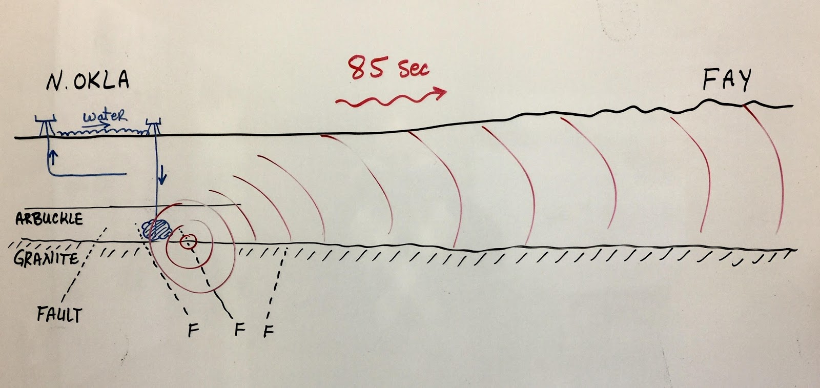 |
| Sketch of NE OK earthquake as felt in Fayetteville, AR |